Intro to Active Preference Learning for Reward Functions in Reinforcement Learning (RL)

Using an active preference-based Gaussian process (GP) regression technique to learn reward functions.

Published by: Alishba Imran

Co-edited by: Anson Leung, William Ngo

The goal of this blog is to explain how we can efficiently learn reward functions while encoding a human’s preference for how any dynamical system (a machine, robot, etc.) should act. Specifically, I will be looking at how an active preference-based Gaussian process regression technique can be used to learn reward functions.  

Markov Decision Processes (MDPs)

Before we get into this, I wanted to do a quick recap on the key concepts behind RL. Markov Decision Processes (MDPs) are mathematical frameworks to describe an environment in reinforcement learning and are often used to formalize RL problems.  An MDP consists of a set of environment states S, a set of possible actions A(s) in each state, a real-valued reward function R(s, a) that depends on the action taken or R(s, a, s') that depends on the action taken and outcome state. As well as a transition model P(s’, s | a). The agent is essentially working to take different actions to try and maximize rewards. 

Reward Functions for High-DOF Robot Arm Motion

Let’s say you have a task where you have a user that wants a robot to learn from a task. The user knows the internal reward function that they want the robot to learn but the robot doesn’t know this reward function. It’s very difficult to teleoperate especially in tasks with very high degrees of freedom. These are often the types of tasks (with high-DOF) that you are dealing with in robotics.

Defining a reward function is a complex task

The success of RL applications depends heavily on the prior knowledge that is put into the definition of the reward function. Although a reward function is a transferable and compact definition of the learning task, the learned policy is usually sensitive to small changes of the reward, which can lead to very different behaviors, depending on the relative values of the rewards. This is why the choice of the reward function has a crucial impact on the success of the learner and many tasks, in particular in robotics that require a high amount of reward engineering.

There are four main problems that lead to difficulties in reward engineering:

(1) Reward Hacking: The agent may maximize the given reward, without performing the intended task. 

(2) Reward Shaping: In many applications, the reward does not only define the goal but also guides the agent to the correct solution, which is also known as reward shaping. Striking a balance between the goal definition and the guidance task is also often very difficult for the experimenter. 

(3) Infinite rewards: Some applications require infinite rewards, for instance, if certain events should be avoided at any cost. 

(4) Multi-objective trade-offs: If it is required to aggregate multiple numeric reward signals, a trade-off is required but the trade-off may not be explicitly known. This is why different parameterizations have to be evaluated for obtaining a policy that correlates with the expected outcome.

Preference-Based Learning

Lets look at a specific example where the user wants the robot to play a variant of mini-golf. But the targets that you see on the ground have different squares and shapes. The user knows these squares but the robot doesn’t. This is where preference-based learning can be useful. The robot shows the user various trajectories to which the user can select and pick which trajectories they prefer to accomplish the given task. 

A lot of prior work in this space assumed that reward functions are linear in some trajectory features. These trajectory features are test-specific. For example, in the mini-golf task, the distance of the balls from the target might be the features. But you can’t just learn these weights because these features are incredibly difficult to design. These are important because if the features are not well designed, then the system can totally fail.

In this mini-golf task, it should be sufficient to have the shot speed and shot angle as our trajectory features that will successfully hit the ball into one of the targets. But with linear rewards, the optimal shot is going to end up in either of the four blue quadrants (shown below) because the robot will try to either maximize or minimize the speed and the angle. We could keep the linear function if we defined if features for each and every target to represent equal distance between the wall and our target. But this approach is not scalable. 

Instead, we want to model the reward as a non-linear function of features that will allow for the optimal behavior to correspond with any point in this highlighted region (shown below). If you can learn such a non-linear function, then the feature design will not be as difficult because the reward function will handle it. 

It is difficult for people to provide demonstrations of the desired system trajectory (like a high-DOF robot arm motion), or to even assign how much numerical reward an action or trajectory should get. This is where preference-based learning can be used where the person provides the system a relative preference between two trajectories.

The learned reward function strongly depends on what environments and trajectories were experienced during the training phase. This can be solved using active learning where the system decides on what preference queries to make. We’ve also found that with active learning, the algorithm converges faster to the desired reward. 

Passive RL vs. Active RL

Before I get into how we can model this reward function, it’s important to understand the main differences between passive RL and active RL, as well as why active RL makes more sense to solve this problem. 

Passive RL

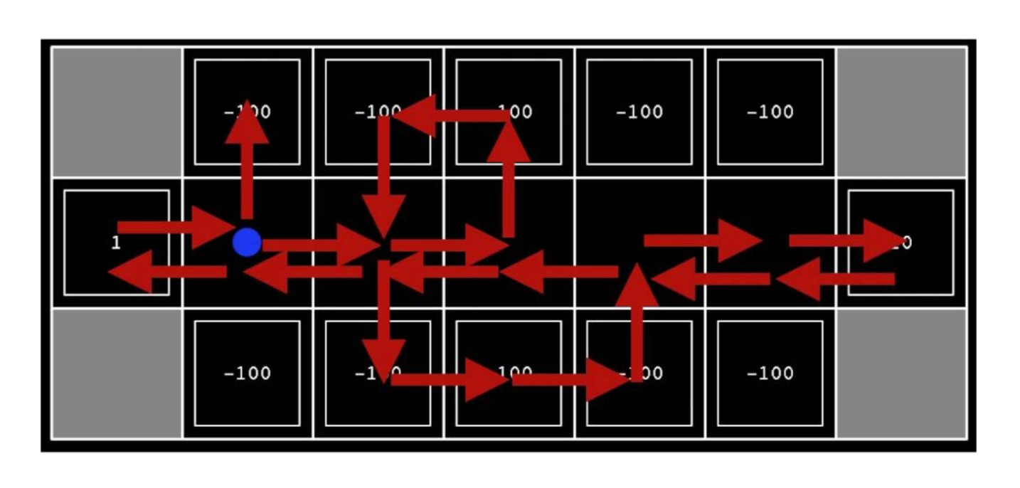
Let’s take a look at the image shown below: we see all the reward values for all the states on the screen. As an agent exploring this environment, the agent doesn’t have access to even the rewards that we’re seeing. What it has access to are the direct interactions with the environment. So it can try random actions to take different paths (shown by the different directions of the arrows). The idea is that we’re considering an algorithm whose input is going to be a history of what the agent tried to do (actions they took), resulting transitions that occurred and the rewards that came with those actions and transitions. If we are able to learn a good policy or utility function or something about the environment, then what we’ve done is Passive RL. 

Passive RL Key Areas

1. Direct Utility Estimation (thought experiment): The algorithm gets recordings of an agent that’s running a fixed policy. Essentially we are watching this agent try to get rewards in some environment by running a policy. We can then go in and use the rewards, the state transitions, the actions that we know the policy was trying to execute, and then attempt to estimate the utility function. An agent's utility function is defined in terms of the agent's history of interactions with its environment. Essentially we treat each time step, each action taken in the recordings, as an example of what the future rewards will be and then we just directly estimate the utility using those samples.  

2. Adaptive Dynamic Programming: this is essentially an estimation of the transition probabilities. The transition probability can be defined as the probability that the agent will move from one state to another. And then running policy iteration on top of that using our estimated rewards and estimated transition probabilities.

3. Temporal-difference (TD) learning: this is a strategy that updates our current estimates of the utilities every single time that we make a transition where we take an action or end up in a new or same state. We then compare the estimated utility of the state that we are in vs. the state that we transitioned to. We treat that as a sample of what we think our current expected future utility or reward is going to be and we compare that to our current estimate. If that’s bigger than it should be then we increase our estimate but if it’s smaller than it should be then we decrease our estimate. 

Problems with Passive RL

There isn’t a good way to update the policy even after we estimate the utilities because we don’t know the transition probabilities (this is at least the case with direct utility estimation). And with ADP we’re estimating the transition probabilities but we don’t have a very good estimate because all we’re sampling are the transitions that happen when we take the actions according to our fixed policy. This means that we have a very limited sample of what the transitions will be for any action that’s not in that original fixed policy. We’re estimating utilities that are represented by the U’s. We have a good idea that we can estimate these utilities pretty well from these passive recordings of the agent running around in the environment. But we can only get a good estimate of the transition probabilities for the actions in our policy (which is fixed). So we can’t estimate the transition probabilities for any action that isn’t in our policy. 

Active RL: Exploration vs. Exploitation 

Within active RL, we now have the ability to choose the actions for the agents to try, and that gives us the opportunity to try actions that aren’t in our policy. Active RL is all about Exploration vs. Exploitation. Exploitation is just a term for using the best policy that we have right now. Exploration is the opposite. Not using the best policy we have right now, with the common approach to exploration being just to choose actions randomly. That works fine in some situations but it can be a very bad idea in other situations. To be more efficient, you can also shrink the probability of that random action over time. This means that most of the time you’re gonna take the optimal policy (so you get good rewards) but in unknown states, you will likely take random actions as well. But if you’ve already visited that state then you’d essentially want to take that random action not as often. 

One way to do this is to always try to use our current estimates of transition probabilities and utilities to pick the action that will give us the highest future reward. You won’t estimate the true utility (it will be an overly optimistic one). U+ on the image below represents the overestimated utility. N represents the number of times we’ve tried out the transition ‘a’ from state ‘s’. The ‘f’ is going to be a function that tells you how much you should trust the current estimate of your utility. And if you don’t trust the current estimate of your utility then we can use an overestimate (assume that there will be a great reward if we try that action). 

Active Preference-Based Gaussian Process (GP) Regression 

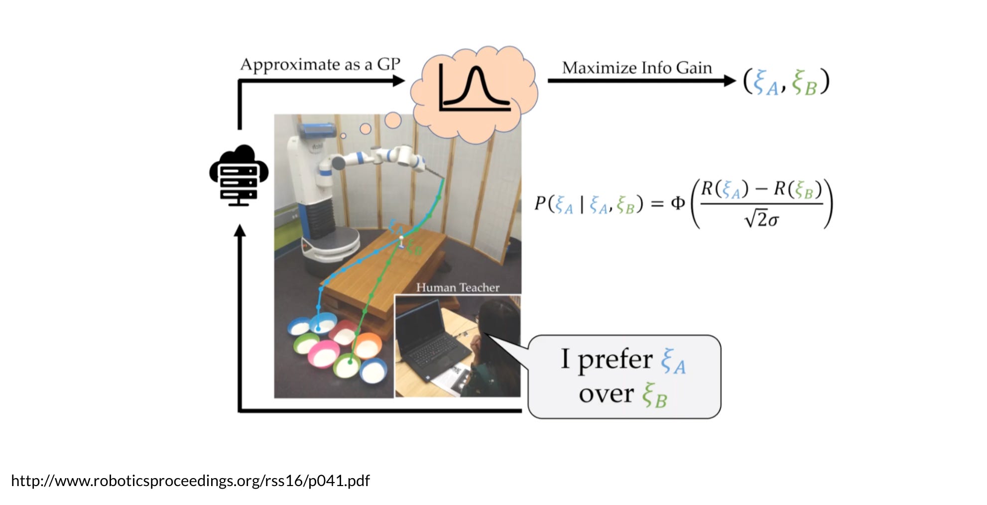
To model the reward function we can use Gaussian processes because they can be more efficiently used with a small number of datasets. This idea represents work presented in this paper.  We want to improve our data efficiency as much as possible because every query gives at most 1 bit of information. This is why on top of using Gaussian processes, you have to actively generate the queries to maximize the information gain. 

The robot will keep a Gaussian process, using this model it will generate the pair of trajectories that will give the highest expected information gain. The robot will show the trajectories to the user who will then respond to the query. This response is stored in a database. Here they used the probit model for human responses. Depending on how close the rewards are to each other this model produces probabilities that are close or different. Using this model, the dataset will give a likelihood function that can be used for fitting the GP. If it doesn’t fall into the class of GPs, then the GP can be approximated.

Some future questions that I have about using a Gaussian process > Neural networks to model the reward function is how scalable Gaussian processes can be past just a few examples.

More Resources

I touched just the tip of exciting research going on in this space. If you’re interested to dive deeper into the math, I would recommend checking out these two papers “Batch Active Preference-Based Learning of Reward Functions” and “Active Preference-Based Learning of Reward Functions” to learn more!

---

Thanks for checking out this blog! If you’re interested in keeping up with future pieces we write, please consider subscribing.

About Us

Welcome to ML Reading Group! We’re a group of students, researchers, and developers sharing our learnings from the latest ML and robotics research papers on topics such as Bayesian Optimization, Active Learning, Reinforcement Learning, Imitation Learning, Time Series Models, and much more!

Our group currently consists of:

• Alishba Imran: worked as an ML Developer at Hanson Robotics to develop Neuro-Symbolic AI, RL, and Generative Grasping CNN approaches for Sophia the Robot. Applied this work with a masters student and professor at San Jose State University, with support from the BLINC Lab, to reduce cost of prosthetics from $10k to $700, and make grasping more effecient. Currently, the co-founder of Voltx and working on RL and Imitation Learning techniques for machine manipulation tasks at Kindred.Ai.

• William Ngo: previously worked as a Research Intern at Canada Excellence Research Chair to apply Deep Learning methods to help solve mathematical optimization problems. Also worked as a Data Science Consultant at Omnia AI, Deloitte Canada's AI Practice. Currently, an MSc Computer Science Student at the University of Toronto and an AI Engineering Intern at Kindred.Ai.

• Anson Leung: worked on a cloud computing platform and recognition computing at IBM, and as a Software Engineer at Oursky. Currently, completing his MSc in Applied Computing at the University of Toronto.

You can get in touch with us here anytime:

• Alishba Imran: Email, LinkedIn, Twitter.

• Anson Leung: Email, LinkedIn.

• William Ngo: Email, LinkedIn.